Examples
This page has a few examples to get you familiar with Starplot and how it works.
- Star Chart for Time/Location
- Star Chart with More Detail
- Map of Orion
- Map of The Pleiades with a Scope Field of View
- Optic plot of The Pleiades with a Refractor Telescope
- Map of The Big Dipper with Custom Markers
- Map of Hale-Bopp in 1997
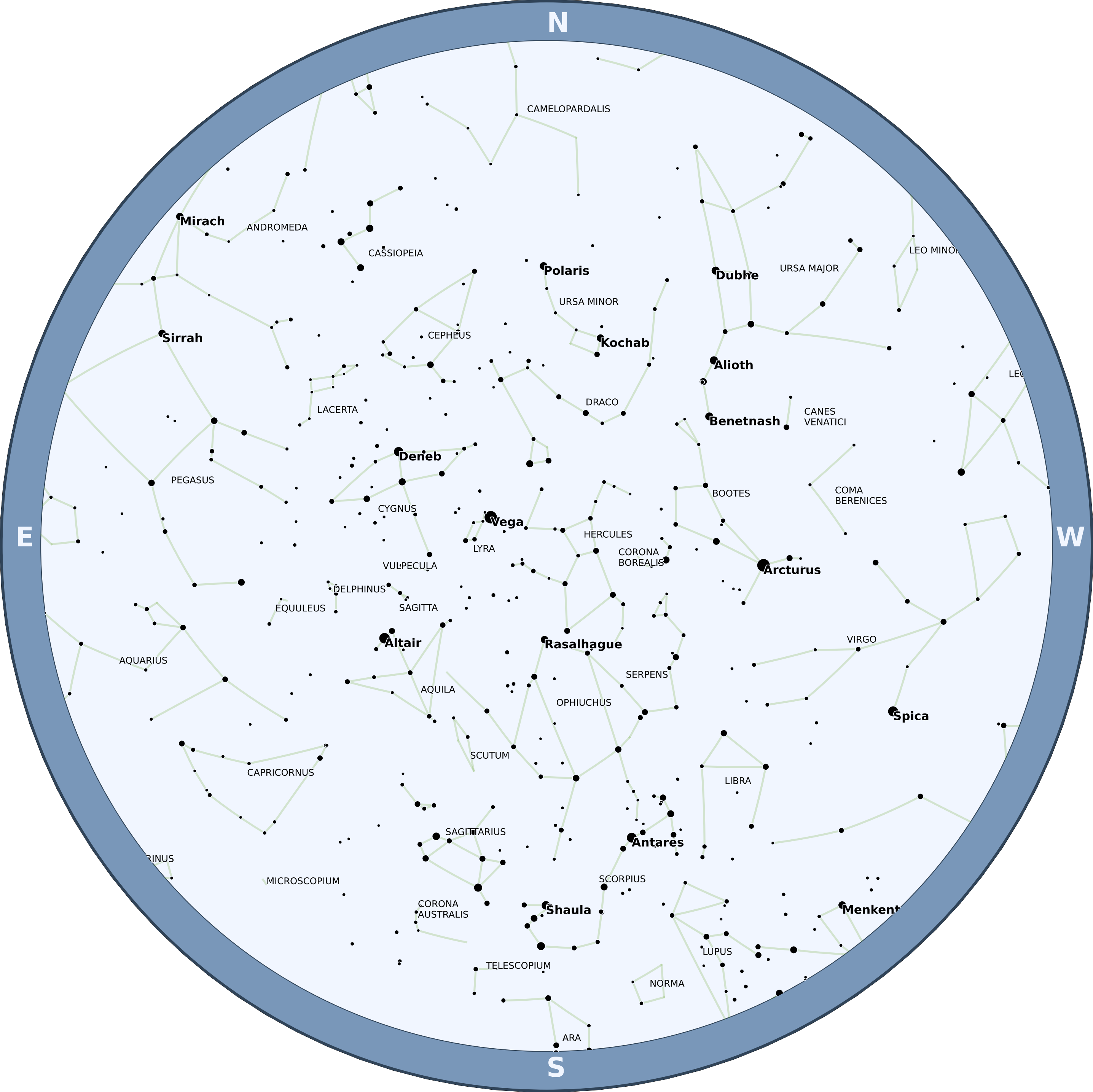
Star Chart for Time/Location
To create a star chart for the sky as seen from Palomar Mountain in California on July 13, 2023 at 10pm PT:
from datetime import datetime
from pytz import timezone
from starplot import MapPlot, Projection
from starplot.styles import PlotStyle, extensions

tz = timezone("America/Los_Angeles")
dt = datetime(2023, 7, 13, 22, 0, tzinfo=tz)  # July 13, 2023 at 10pm PT

p = MapPlot(
    projection=Projection.ZENITH,
    lat=33.363484,
    lon=-116.836394,
    dt=dt,
    style=PlotStyle().extend(
        extensions.BLUE_MEDIUM,
        extensions.ZENITH,
    ),
    resolution=2600,
)
p.constellations()
p.stars(mag=4.6, mag_labels=2.1)

p.export("01_star_chart.png", transparent=True)
The created file should look like this:
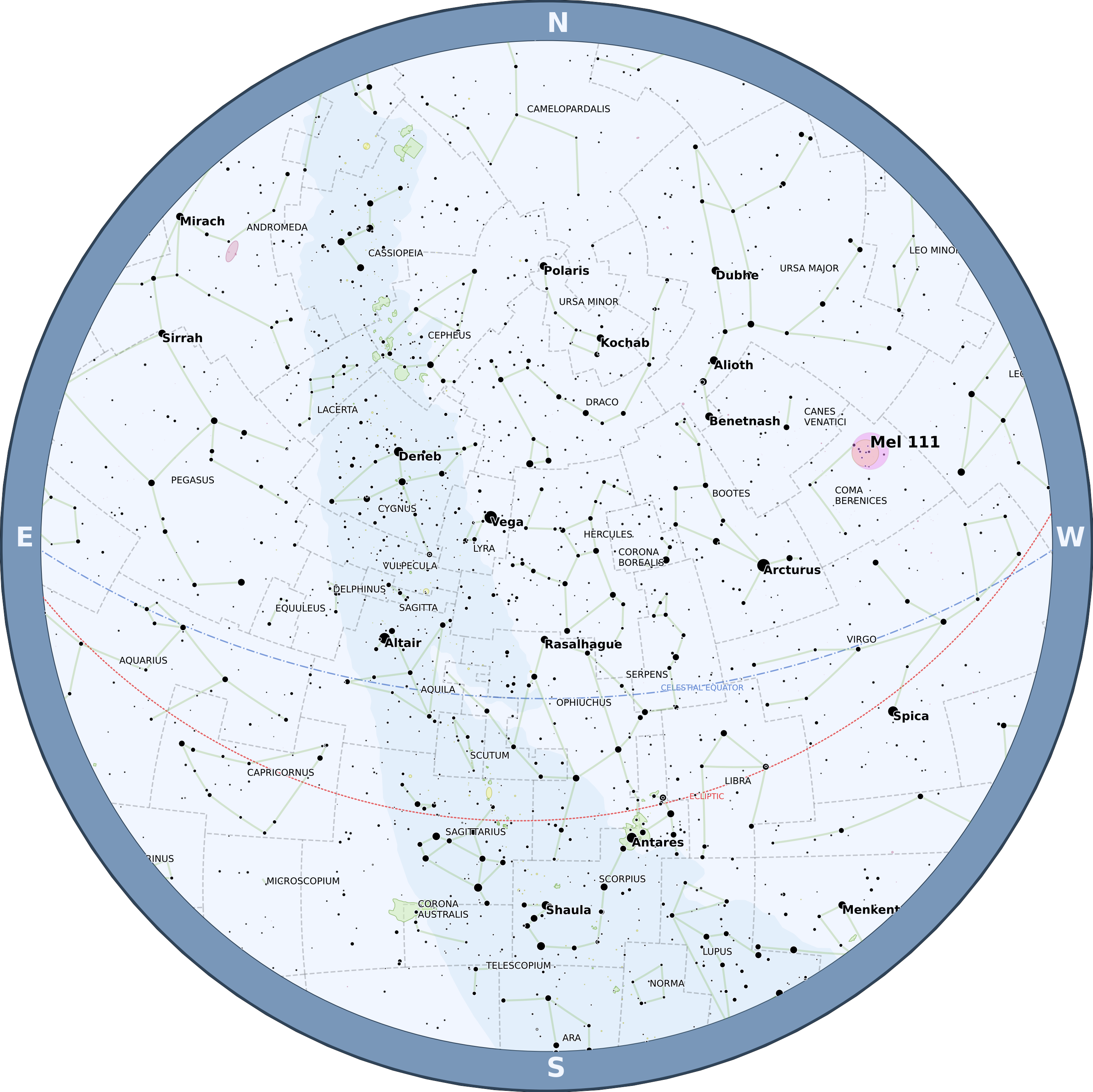
Star Chart with More Detail
Building on the first example, you can also plot additional objects and even customize their style. Here's an example that plots a bunch of extra stuff (including the Milky Way, constellation borders, Deep Sky Objects, and more). It also demonstrates how you can plot your own markers, like the purple circle around the Coma Star Cluster (Melotte 111):
from datetime import datetime
from pytz import timezone
from starplot import MapPlot, Projection
from starplot.styles import PlotStyle, extensions

tz = timezone("America/Los_Angeles")
dt = datetime(2023, 7, 13, 22, 0, tzinfo=tz)  # July 13, 2023 at 10pm PT

p = MapPlot(
    projection=Projection.ZENITH,
    lat=33.363484,
    lon=-116.836394,
    dt=dt,
    style=PlotStyle().extend(
        extensions.BLUE_MEDIUM,
        extensions.ZENITH,
    ),
    resolution=2600,
)
p.constellations()
p.stars(mag=5.6, mag_labels=2.1)

p.dsos(mag=9, null=True, true_size=True, labels=None)
p.constellation_borders()
p.ecliptic()
p.celestial_equator()
p.milky_way()

p.marker(
    ra=12.36,
    dec=25.85,
    label="Mel 111",
    style={
        "marker": {
            "size": 28,
            "symbol": "circle",
            "fill": "full",
            "color": "#ed7eed",
            "edge_color": "#e0c1e0",
            "alpha": 0.4,
            "zorder": 100,
        },
        "label": {
            "zorder": 200,
            "font_size": 12,
            "font_weight": "bold",
        },
    },
)

p.export("02_star_chart_extra.png", transparent=True)
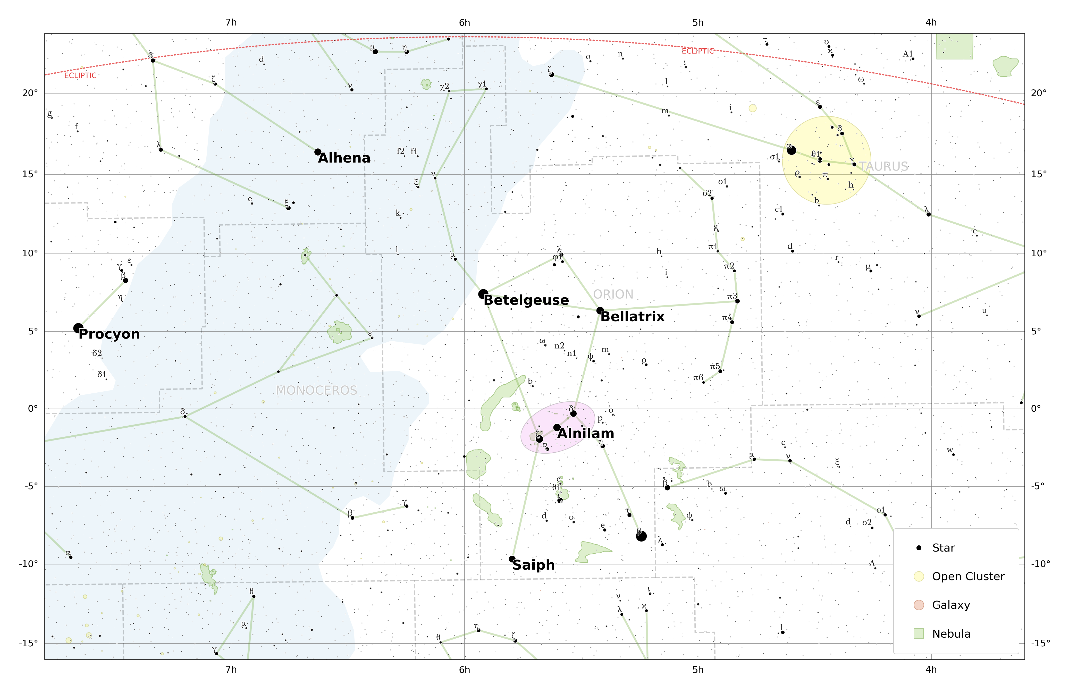
Map of Orion
The following code will create a simple map plot that shows the area around the constellation Orion, including a legend and an ellipse around Orion's Belt:
from starplot import MapPlot, Projection
from starplot.styles import PlotStyle, PolygonStyle, extensions

style = PlotStyle().extend(
    extensions.BLUE_LIGHT,
    extensions.MAP,
    {
        "bayer_labels": {
            "font_name": "GFS Didot",  # use a better font for Greek letters
            "font_size": 7,
            "font_alpha": 0.9,
        },
        "legend": {
            "location": "lower right",  # show legend inside map
            "num_columns": 1,
            "background_alpha": 1,
        },
    },
)

p = MapPlot(
    projection=Projection.MERCATOR,
    ra_min=3.6,
    ra_max=7.8,
    dec_min=-16,
    dec_max=23.6,
    style=style,
    resolution=3600,
)
p.gridlines()
p.stars(mag=9, bayer_labels=True)
p.dsos(mag=9, null=True, labels=None)
p.constellations()
p.constellation_borders()
p.milky_way()
p.ecliptic()

p.ellipse(
    (5.6, -1.2),
    height_degrees=3,
    width_degrees=5,
    style=PolygonStyle(
        fill_color="#ed7eed",
        edge_color="#000",
        alpha=0.2,
    ),
    angle=-22,
)

p.legend()

p.export("03_map_orion.png", padding=0.5)
The result should look like this:
Map of The Pleiades with a Scope Field of View
The following code will create a minimal map plot that shows the field of view (red dashed circle) of The Pleiades (M45) when looking through a Tele Vue 85 telescope with a 14mm eyepiece that has a 82 degree FOV:
from starplot import MapPlot, Projection
from starplot.styles import PlotStyle, extensions

style = PlotStyle().extend(
    extensions.GRAYSCALE,
    extensions.MAP,
)
style.star.marker.size = 60

p = MapPlot(
    projection=Projection.STEREO_NORTH,
    ra_min=54.5 / 15,
    ra_max=58.5 / 15,
    dec_min=22.5,
    dec_max=25.5,
    style=style,
    resolution=1400,
)
p.stars(
    mag=14,
    catalog="tycho-1",
)
p.dsos(mag=8, labels=None)
p.scope_fov(
    ra=3.7912778,
    dec=24.1052778,
    scope_focal_length=600,
    eyepiece_focal_length=14,
    eyepiece_fov=82,
)
p.title("M45 :: TV-85 / 14mm @ 82deg")
p.export("04_map_m45_scope.png", padding=0.3)
The result should look like this:
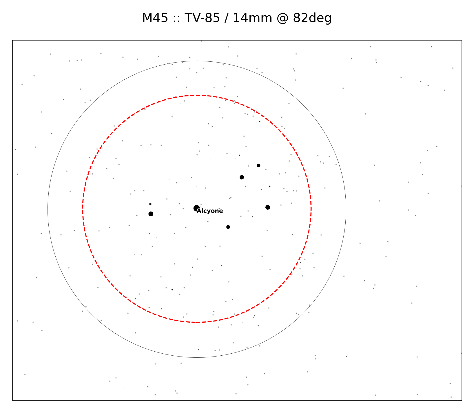
The solid black circle in this plot is the extent of the Pleiades as defined in OpenNGC.
Binocular Field of View
You can also plot a circle showing the field of view of binoculars with the bino_fov function:
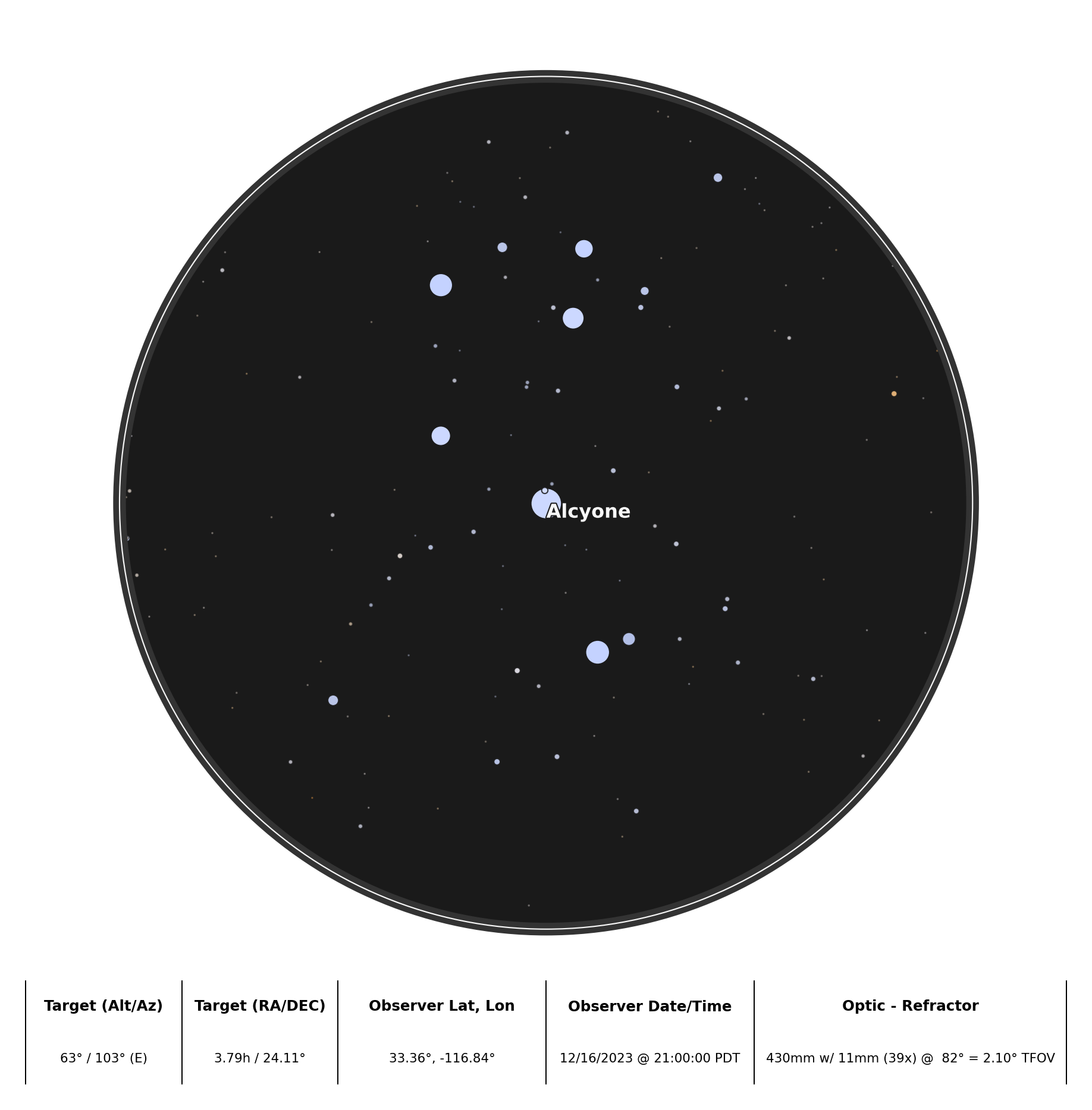
Optic Plot of The Pleiades with a Refractor Telescope
The following code will create an optic plot that shows what The Pleiades looked like through a refractor telescope on December 16, 2023 at 9pm PT from Palomar Mountain in California.
from datetime import datetime
from pytz import timezone
from starplot import OpticPlot
from starplot.callables import color_by_bv
from starplot.optics import Refractor
from starplot.styles import PlotStyle, extensions

dt = datetime.now(timezone("US/Pacific")).replace(2023, 12, 16, 21, 0, 0)

style = PlotStyle().extend(
    extensions.GRAYSCALE_DARK,
    extensions.OPTIC,
)

p = OpticPlot(
    # M45
    ra=3.7912778,
    dec=24.1052778,
    lat=33.363484,
    lon=-116.836394,
    # Refractor Telescope
    optic=Refractor(
        focal_length=430,
        eyepiece_focal_length=11,
        eyepiece_fov=82,
    ),
    dt=dt,
    style=style,
    resolution=1600,
)
p.stars(
    mag=12,
    color_fn=color_by_bv,
)
p.info()
p.export("05_optic_m45.png", padding=0.3)
The result should look like this:
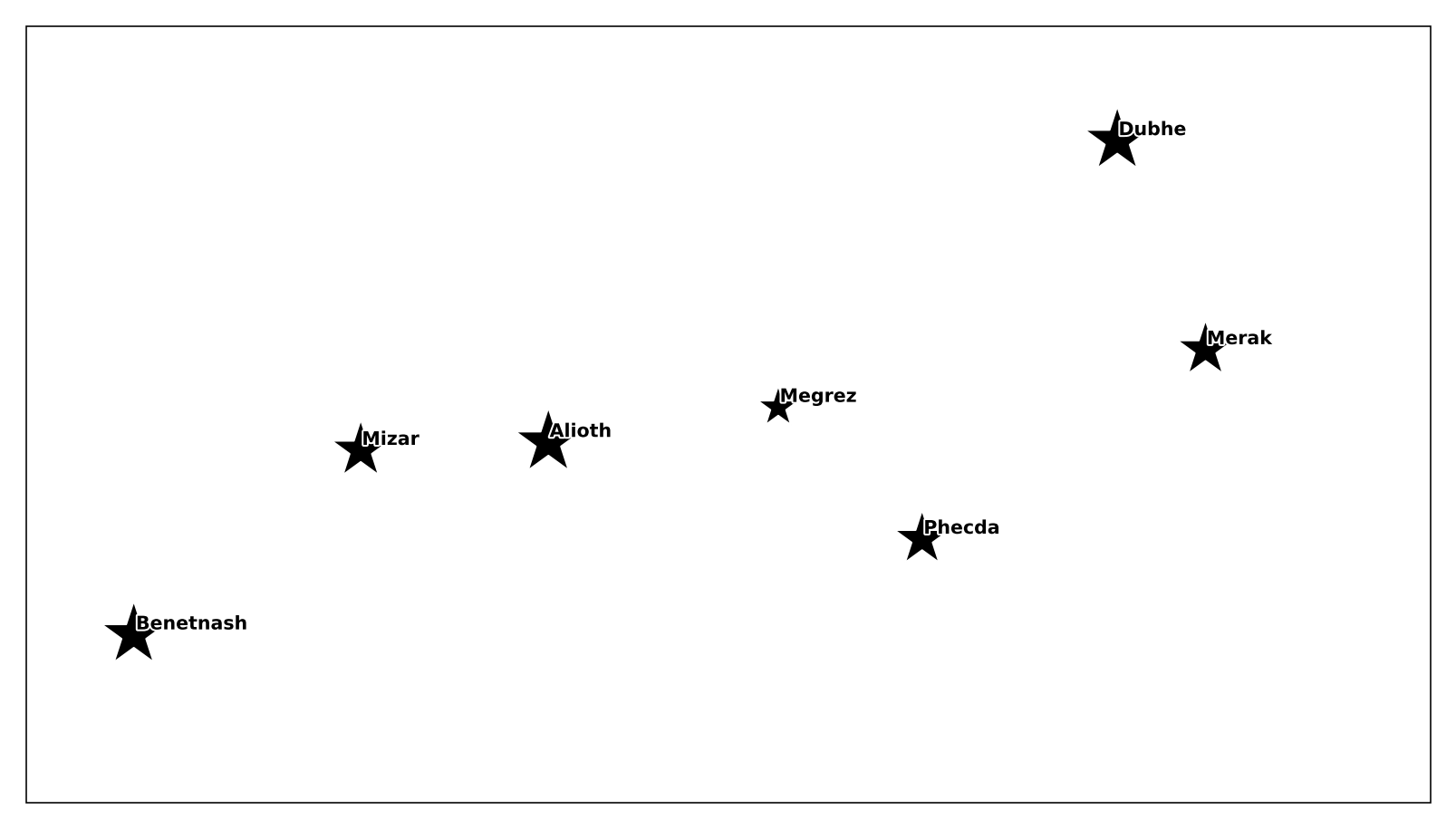
Map of The Big Dipper with Custom Markers
Here's a fun one 😃 Let's create a small plot of the big dipper (Ursa Major), but with custom star-shaped markers:
from starplot import MapPlot, Projection
from starplot.styles import PlotStyle, extensions, MarkerSymbolEnum

style = PlotStyle().extend(
    extensions.GRAYSCALE,
    extensions.MAP,
)

style.star.marker.symbol = MarkerSymbolEnum.STAR

# By default, star sizes are calculated based on their magnitude first,
# but then that result will be multiplied by the star's marker size in the PlotStyle
# so, adjusting the star marker size is a way to make all stars bigger or smaller
style.star.marker.size = 80

p = MapPlot(
    projection=Projection.STEREO_NORTH,
    ra_min=10.8,
    ra_max=14,
    dec_min=48,
    dec_max=64,
    style=style,
    resolution=1400,
)
p.stars(mag=3.6)
p.adjust_text()
p.export("06_big_dipper_stars.png", padding=0.2)
The result should look like this:
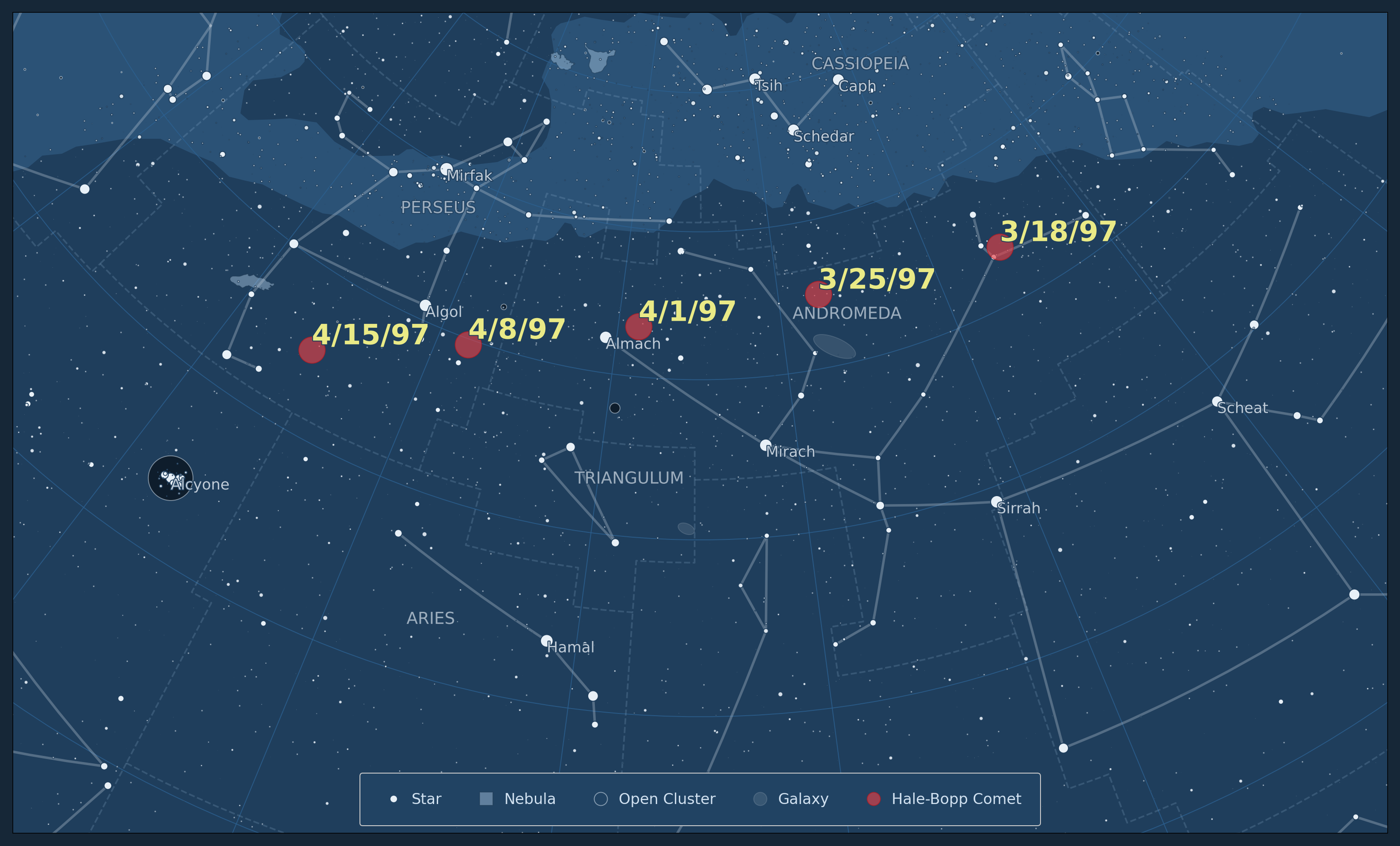
Map of Hale-Bopp in 1997
Here's an example that uses Skyfield to get some data on the comet Hale-Bopp ☄️ and then uses that data to plot the comet's location in the sky in March and April of 1997 (when the comet was at its brightest in the sky):
Note
Skyfield is a required dependency of Starplot (and a very important one!), so if you have Starplot installed, then Skyfield should be installed too.
from skyfield.api import load
from skyfield.data import mpc
from skyfield.constants import GM_SUN_Pitjeva_2005_km3_s2 as GM_SUN

from starplot import MapPlot, Projection
from starplot.styles import PlotStyle, extensions

# First, we use Skyfield to get comet data
# Code adapted from: https://rhodesmill.org/skyfield/kepler-orbits.html#comets
with load.open(mpc.COMET_URL) as f:
    comets = mpc.load_comets_dataframe(f)

# Keep only the most recent orbit for each comet,
# and index by designation for fast lookup.
comets = (
    comets.sort_values("reference")
    .groupby("designation", as_index=False)
    .last()
    .set_index("designation", drop=False)
)

# Find Hale-Bopp
row = comets.loc["C/1995 O1 (Hale-Bopp)"]

ts = load.timescale()
eph = load("de421.bsp")
sun, earth = eph["sun"], eph["earth"]
comet = sun + mpc.comet_orbit(row, ts, GM_SUN)

# Find the RA/DEC of comet for every 7 days starting on March 18, 1997
radecs = []
for day in range(0, 30, 7):
    t = ts.utc(1997, 3, 18 + day)
    ra, dec, distance = earth.at(t).observe(comet).radec()
    radecs.append((t, ra.hours, dec.degrees))

# Now let's plot the data on a map!
style = PlotStyle().extend(
    extensions.BLUE_DARK,
    extensions.MAP,
    {
        "star": {
            "label": {
                "font_size": 9,
                "font_weight": "normal",
            }
        },
        "legend": {
            "location": "lower center",
        },
    },
)
style.legend.location = "lower center"

p = MapPlot(
    projection=Projection.STEREO_NORTH,
    # to make plots that are centered around the 0h equinox, you can
    # set the max RA to a number over 24 which will determine how
    # far past 0h the plot will extend. For example, here we set
    # the max RA to 28, so this plot will have an RA extent from 23h to 4h
    ra_min=23,
    ra_max=28,
    dec_min=14,
    dec_max=60,
    style=style,
    resolution=2800,
)
p.gridlines(labels=False)
p.stars(mag=8)
p.constellations()
p.constellation_borders()
p.nebula(mag=8, labels=None)
p.open_clusters(mag=8, labels=None)
p.galaxies(mag=8, labels=None)
p.milky_way()

for t, ra, dec in radecs:
    label = f"{t.utc.month}/{t.utc.day}/{t.utc.year % 100}"
    p.marker(
        ra=ra,
        dec=dec,
        label=label,
        legend_label="Hale-Bopp Comet",
        style={
            "marker": {
                "size": 16,
                "symbol": "circle",
                "fill": "full",
                "color": "hsl(358, 78%, 58%)",
                "edge_color": "hsl(358, 78%, 42%)",
                "alpha": 0.64,
                "zorder": 4096,
            },
            "label": {
                "font_size": 17,
                "font_weight": "bold",
                "font_color": "hsl(60, 70%, 72%)",
                "zorder": 4096,
            },
        },
    )

p.legend()

p.export("07_map_hale_bopp.png", padding=0.2)
The result should look like this:
Check out the code reference to learn more about using starplot!